Reconstructing mult-omics networks with coglasso • coglasso

Introduction

This vignette illustrates the basic usage of the coglasso package to reconstruct a multi-omics network. The package implements an R interface to collaborative graphical lasso (Albanese, Kohlen and Behrouzi, 2024), a network estimation algorithm based on graphical lasso (Friedman, Hastie and Tibshirani, 2008) and collaborative regression (Gross and Tibshirani, 2015)

Let us first attach coglasso.

library(coglasso)

We then choose the multi-omics data set to use. The coglasso package offers three alternative version of a transcriptomics and metabolomics data set. We will use multi_omics_sd_small. For further explanation about the available multi-omics data sets see help(multi_omics_sd).

colnames(multi_omics_sd_small)
#>  [1] "Cirbp"       "Hspa5"       "P4ha1"       "Spred1"      "Creld2"     
#>  [6] "Pdia6"       "Hsp90b1"     "Hsph1"       "Manf"        "Pdia3"      
#> [11] "Dnajb11"     "Dnajc3"      "BC004004"    "Stip1"       "Phe"        
#> [16] "Trp"         "Putrescine"  "PC aa C36:3" "PC ae C32:2"
nrow(multi_omics_sd_small)
#> [1] 30

This smaller version of multi_omics_sd has 19 variables, 14 genes and 5 metabolites, and 30 samples. We can directly proceed with network reconstruction.

Multi-omics network reconstruction

Our objective is to reconstruct a network from this data set using collaborative graphical lasso. To do so with the coglasso package, we mainly call a function: bs(). This function first estimates a network for every combination of hyperparameters we want to explore, then it selects the best combination according to the chosen model selection method.

The usual application of bs() requires to give an input data set to the argument data, the number of variables of the various omics layers p, and the hyperparameter settings. Collaborative graphical lasso has three hyperparameters: $λ_w$ , penalizing “within” same-type interactions, $λ_b$ penalizing “between” different-type interactions, and $c$ , the weight of the collaborative term. In this vignette we choose to explore 15 possible penalty values for both “within” and “between” penalties, and three possible collaboration values. We do so by setting both nlambda_w and nlambda_b to 15, and by setting nc to 3. We also decide to focus our search to the sparse side of possible “within” networks. We achieve this by setting to a fixed value the ratio between the smallest (least penalizing) and the largest (most penalizing) $λ_w$ explored. While the default value of these parameter is 0.1 for both $λ_w$ and $λ_b$ , we decide to set the minimum ratio to 0.6 for $λ_w$ .

It is also possible to set options for the model selection procedure, if one does not want to enjoy the comfort of the default behaviour. To select the best combination of hyperparameters, we will set method to “xestars” (which is the default behaviour). This implements eXtended Efficient StARS, a significantly faster version of eXtended StARS (XStARS, Albanese, Kohlen and Behrouzi, 2024). XEStARS and XStARS are a coglasso-adapted version of StARS, the stability selection method developed by Liu, Roeder and Wasserman (2010). The suggested application of bs() uses the default options of the function. For further explanation on other selection methods available, and on other arguments of bs() and how to use them, please see help(bs).

sel_cg <- bs(
  multi_omics_sd_small,
  p = c(14, 5),
  nlambda_w = 15,
  nlambda_b = 15,
  nc = 3,
  lambda_w_min_ratio = 0.6,
  verbose = FALSE
)

# To see information on the network estimation and selection:
print(sel_cg)
#> Selected network estimated with collaborative graphical lasso
#> 
#> The call was:
#> bs(data = multi_omics_sd_small, p = c(14, 5), nlambda_w = 15, 
#>     nlambda_b = 15, nc = 3, lambda_w_min_ratio = 0.6, verbose = FALSE)
#> 
#> The model selection method was:
#> xestars
#> The density of the selected network is:
#> 0.01169591
#> 
#> Networks are made of 2 omics layers, for a total of 19 nodes
#> For each layer they have: 14 and 5 nodes, respectively
#> 
#> The selected value for lambda within is:
#> 0.9137
#> The selected value for lambda between is:
#> 0.5024
#> The selected value for c is:
#> 3.1623
#> 
#> The total number of hyperparameter combinations explored was:
#> 675
#> The values explored for lambda within were:
#> 0.9137, 0.881, 0.8494, 0.819, 0.7896, 0.7613, 0.734, 0.7077, 0.6824, 0.6579, 0.6344, 0.6116, 0.5897, 0.5686, 0.5482
#> The values explored for lambda between were:
#> 0.5922, 0.5024, 0.4262, 0.3615, 0.3067, 0.2602, 0.2207, 0.1873, 0.1589, 0.1348, 0.1143, 0.097, 0.0823, 0.0698, 0.0592
#> The values explored for c were:
#> 10, 3.1623, 1
#> 
#> Plot the selected network with:
#> plot(sel_cg)

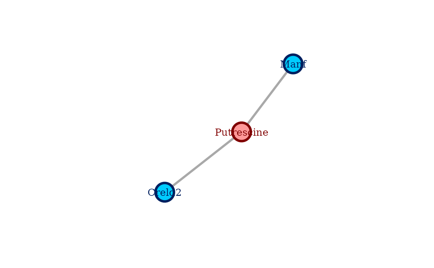
With this we have fast selected the combination of hyperparameters yielding the most stable, yet sparse coglasso network. We can directly plot the selected network with:

plot(sel_cg)

References

Albanese, A., Kohlen, W., & Behrouzi, P. (2024). Collaborative graphical lasso (arXiv:2403.18602). arXiv https://doi.org/10.48550/arXiv.2403.18602

Friedman, J., Hastie, T., & Tibshirani, R. (2008). Sparse inverse covariance estimation with the graphical lasso. Biostatistics, 9(3), 432–441. https://doi.org/10.1093/biostatistics/kxm045

Gross, S. M., & Tibshirani, R. (2015). Collaborative regression. Biostatistics, 16(2), 326–338. https://doi.org/10.1093/biostatistics/kxu047

Liu, H., Roeder, K., & Wasserman, L. (2010). Stability Approach to Regularization Selection (StARS) for High Dimensional Graphical Models (arXiv:1006.3316). arXiv https://doi.org/10.48550/arXiv.1006.3316