Reconstruct and analyse multi-omics networks with carmon

Introduction

Copula-Aided Reconstruction of Multi-Omics Networks () is an R package empowered by the use of copulas as a statistical tool for the reconstruction of multi-omics networks. The use of copulas as a statistical tool allows to transfer raw non-normalized omics data to the normal realm. In this way, the package is able to harness the full statistical power of the information contained in each omics layer of a multi-omics data set. At the same time, the transfer of the multi-omics layer to the normal realm allows the application of network reconstruction models that assume normal distribution of the data. Needless to say, this is an assumption rarely met by omics data, hence a further advantage of the use of copulas. Here, we first cover the formatting of the input data to provide to . Then, we show how to easily build and analyse a multi-omics network with carmon. In the remaining sections, we explore more advanced and customized uses of the package, as well as what actually happens under the hood when the main function carmon() is used.

Installation

You can install from Bioconductor with:

if (!require("BiocManager", quietly = TRUE))
    install.packages("BiocManager")

BiocManager::install("carmon")

Alternatively, you can install the development version from GitHub. First, make sure to install devtools with:

if (!require("devtools")) {
    install.packages("devtools")
}

You can then install the development version with:

devtools::install_github("DrQuestion/carmon")

Input multi-omics data set-up

We first attach the package.

library(carmon)

We can now explain the data format. Carmon expects the input multi-omics data to be arranged in a named R list. Each element of the list should be the data set of one of the omics layers, and it should be preferably named after the omics type it contains. In the package there are several examples of multi-omics data sets of increasing sizes, which you can see with help(multi_omics). Here we use multi_omics_small.

data(multi_omics_small)
str(multi_omics_small)
#> List of 2
#>  $ rnaseq      : num [1:30, 1:14] 1023 815 1047 725 1217 ...
#>   ..- attr(*, "dimnames")=List of 2
#>   .. ..$ : chr [1:30] "BXD100" "BXD101" "BXD73b" "BXD44" ...
#>   .. ..$ : chr [1:14] "Cirbp" "Hspa5" "P4ha1" "Spred1" ...
#>  $ metabolomics: num [1:30, 1:5] 66.1 50.2 56.3 58.9 61 ...
#>   ..- attr(*, "dimnames")=List of 2
#>   .. ..$ : chr [1:30] "BXD100" "BXD101" "BXD73b" "BXD44" ...
#>   .. ..$ : chr [1:5] "Phe" "Trp" "Putrescine" "PC aa C36:3" ...

You can see that this list has two elements, one containing RNA-seq gene counts and named “rnaseq” (multi_omics_small$rnaseq) and the other containing metabolites concentrations and named “metabolomics” (multi_omics_small$metabolomics). Each layer has 30 observations, the first one measuring the expression of 14 genes, the second one the concentration of 5 metabolites. Please notice that carmon expects non-normalized data, to harness at the best the statistical behavior of omics data with copula.

To recreate such an object on R, first it is necessary to make sure that the observations/samples/individuals from which the data set has been measured are in the same order for all the input omics data sets and are consistent in where they are placed for all data sets, either all across the rows or all across the column. For example, in our toy data set, you can see how all the observations are in the same order and distributed along the rows for both the transcriptomic and the metabolomic data set. After your separate data sets are properly formatted, you can assemble them in a single list as follows:

# Let's build two separate data sets just for the sake of our example:
layer_1 <- multi_omics_small$rnaseq
layer_2 <- multi_omics_small$metabolomics

# This shows that observations are on the rows for both data sets:
dim(layer_1) # [1] 30 14
dim(layer_2) # [1] 30  5

# This shows that the observations are all in the same order in both data sets:
all(rownames(layer_1) == rownames(layer_2)) # TRUE

# We can now build our R list as follows:
multi_omics_small <- list("rnaseq" = layer_1, "metabolomics" = layer_2)

Carmon to perform copula-aided reconstruction, analysis and plot of a multi-omics network

The carmon package covers multiple functional steps of network reconstruction and analysis from multi-omics data. To perform a full, default run of carmon, it is necessary to run:

c_obj <- carmon(multi_omics_small)
#> Checking sample-matching, formatting the data,
#>     and other formalities....
#> Done!
#> ****************Beginning copulization****************
#> Copulizing layer 1 of 2 (rnaseq)
#> Copulizing layer 2 of 2 (metabolomics)
#> ****************Copulization complete*****************
#> ***********Beginning network reconstruction***********
#> Reconstructing network with coglasso, selecting the optimal one with xestars....
#> Optimal network selected!
#> ***********Network reconstruction complete************
#> **************Beginning network analysis**************
#> Computing centrality measures....
#> Centrality measures computed!
#> Compiling the report....
#> Report compiled!
#> **************Network analysis complete***************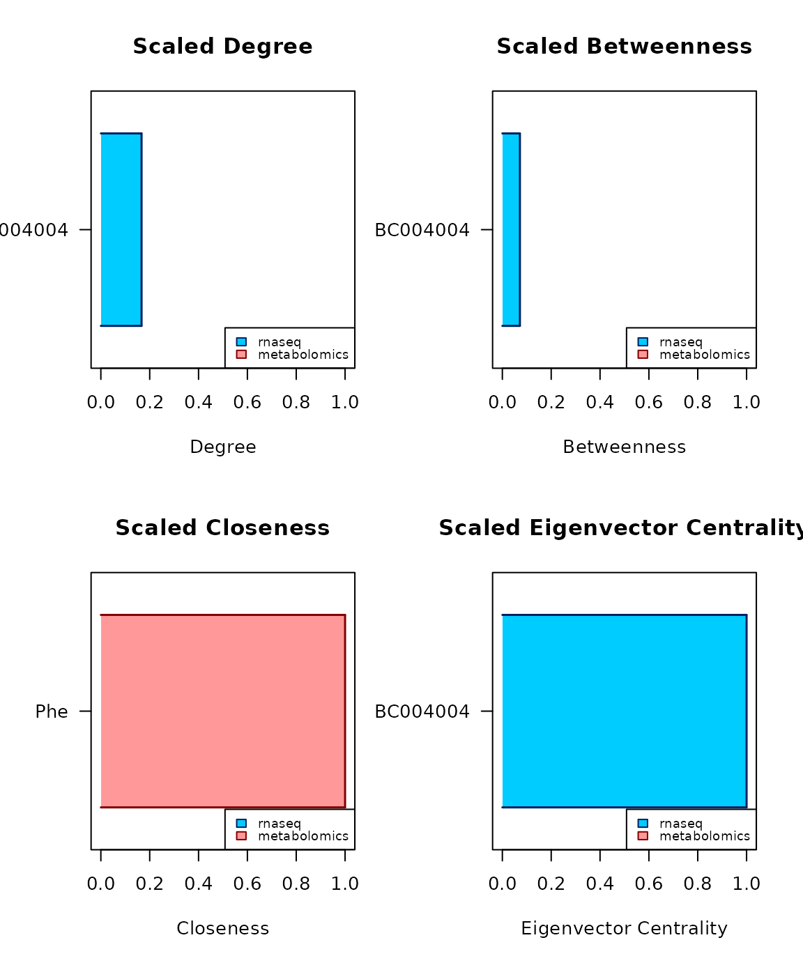

Under the hood, there are several processes happening. In order: the check-ups and formatting of the input data; the copula-based transfer of non-normal omics data to the normal realm; the reconstruction and selection of a multi-omics network; a centrality consensus analysis to identify key components of the network; and the plotting of the multi-omics network (enriched by the information discovered during the centrality analysis) and of the results of the centrality analysis. Most of these steps can be customized within the main wrapper function, using specific arguments. We will see how in the next sections, but first let’s access the results of the centrality consensus analysis with the function centrality_report():

centrality_report(c_obj)
#>          candidate  degree betweenness closeness eigenvector central for
#> BC004004  BC004004 0.1667*     0.0719*       0.6          1*         dbe
#> Phe            Phe  0.1111      0.0065        1*           0           c

Copula-based transfer to the normal realm

Carmon harnesses the raw statistical behavior of the non-normally distributed omics data to perform a proper transfer to the normal realm. The statistical tool the package uses for this task are Gaussian copulas. The first ingredient to perform this transition with copulas is the choice of what statistical behavior best describes your omics data, by deciding which marginal distribution is followed by each omics layer.

The most basic approach to this is to choose the empirical distribution, with which we take the data as they are, without making any assumption. The approach carmon prefers, when possible, is to assume that the data follow specific parametric statistical distributions. With this approach, we use the omics data to estimate the parameters of such distribution, allowing to find the distribution of the chosen family that best describes the omics data.

With specific types of omics data, over the years, the scientific community has settled on specific distributional assumptions. For example, RNA-seq data, together with other omics types that generate count-based measures, are generally assumed to follow a Negative Binomial distribution. Carmon takes several of this known distributional assumptions and implements them as a default to tailor its treatment of those specific omics types. For all those omics types that have no known assumption yet, or those for which we have not tailored a default behavior yet, carmon chooses the first approach, the one based on the assumption-free empirical distribution. To see for which omics types we tailored a default behavior, please use the function which_omics(). Be aware that carmon is built for being upgraded, so soon there will be new omics types for which we implement a tailored default behavior.

which_omics()
#> "rna-seq", also as "rnaseq", "gene counts", "transcriptomics"
#>     is modeled by default as count data with a negative-binomial marginal.
#> 
#> "proteomics", also as "protein fragments", "protein counts"
#>     is modeled by default as count data with a negative-binomial marginal.
#> 
#> "metabolomics", also as "lc-ms", "gc-ms", "ms"
#>     is modeled by default as positive continuous data with a log-normal
#>     marginal.
#> 
#> Anything else is modeled with the empirical marginal.

These are also the terms you can use to name the elements of the input R list if you want to trigger the default behavior for the corresponding layers. For example, you could see that the two elements in the input list multi_omics_small are "rnaseq", which will trigger the default assumption of Negative Binomial distribution to model gene counts, and "metabolomics", which will trigger by default the log-normal distribution to describe the metabolites’ concentrations.

If this is the default behavior for such omics types, but you know that your particular data set follows a different statistical distribution, you can run the function which_marginals(). This function displays which are the statistical distributions that carmon is curently compatible with.

which_marginals()
#> "e" or "empirical" for using the empirical marginal distribution;
#> "n" or "normal" for using the normal marginal distribution;
#> "ln" or "lognormal" for using the log-normal marginal distribution;
#> "nb" or "negative binomial" for using the log-normal marginal distribution.

This information can be used to customize the default behavior of carmon with the copula-based transition to normal data. The two arguments to the main wrapping function carmon() that you can use for this are:

omics: to be provided as a vector of characters, by default it is unnecessary, as the input list will have the omics types in the name given to each element. We recommend its use especially when for some reason the elements are not or cannot be named. An example of it could be when two layers in the list measure the same omics type, so you may want to explicitate it as an input with this argument. This is how you can use it in our example omics = c("rnaseq", "metabolomics").
marginals: also a vector of characters, it overrides the default behavior for the input omics types. It is also possible to have a mixed case, in which for some omics layers you want to trigger the default, and for others you want to customize it. If you know that for your first layer you would rather use the assumption-free empirical distribution, the normal for the second, and you prefer normal behavior for the third, this is the form that the argument could take: marginals = c("e", "n", 0), requesting default behavior with the 0.

Network reconstruction and selection

Once the omics layers have been transferred to the normal realm, carmon() proceeds to build the multi-omics network. For this task the package implements multiple network reconstruction strategies, of which one is chosen. By defualt, the package chooses collaborative graphical lasso (coglasso) (Albanese, Kohlen and Behrouzi, 2024) as its engine to reconstruct the multi-omics network, as the method was specifically developed for the multi-omics network reconstruction scenario. carmon also implements three classic alternatives to the reconstruction of networks: graphical lasso (Friedman, Hastie and Tibshirani, 2008), neighborhood selection (Meinshausen and Buhlmann, 2006), and Pearson’s correlation networks. The network reconstruction strategy can be personalized with the argument net_method, for example net_method = "coglasso", while for choosing one of the other ones, respectively, you would need "glasso", "mb", or "correlation".

Apart from one specific use case, each of these methods explores network reconstruction among a range of hyperparameters, usually resulting in a different network for each different value (or combination of values) these hyperparameters can take. This requires specific model selection procedures that can pinpoint the best network among the ones that have been built. Luckily, for each network reconstruction method it implements, carmon() also comes with its tailored model selection procedures. For coglasso, for example, it is possible to choose among three possible strategies. One of them is the extended Bayesian Information Criterion (eBIC). The other two are different versions of an algorithm based on StARS (Liu, Roeder and Wasserman, 2010), extended to the coglasso case in which three different hyperparameters need to be tuned, and described in (Albanese, Kohlen and Behrouzi, 2024) as XStARS. The two different versions implemented are indeed the original XStARS and the more efficient but slightly less thorough version XEStARS. By default, for coglasso as a network reconstruction method carmon() uses XEStARS. To customize the model selection procedure, you can use the sel_method parameter. For example, if instead of the default you prefer the more thorough XStARS, you can set sel_method = "xstars", with the default being "xestars" and "ebic" being the alternative for using eBIC. For every other network reconstruction procedure, as they are all based on a single hyperparameter, carmon() uses by default the one-dimensional StARS, but more options are available. See them all in help(carmon), under the description of the sel_method argument.

All of the methods mentioned above, either for network reconstruction or network selection, can be further tweaked by giving specific arguments. For example, if using coglasso for reconstruction, and wanting to investigate the hyperparameter space more thoroughly than the default, one could specify the coglasso-specific parameters with a higher number, say nlambda_w = 20 (normally only 8 values are explored), nlambda_b = 20 (only 8 values normally), and nc = 10 (only 5 normally). To see more about these and other arguments one can tweak about coglasso network reconstruction and selection, please see ?coglasso::bs. For the other network reconstruction methods, please see ?huge::huge.glasso for graphical lasso, ?huge::huge.mb for neighborhood selection, and ?huge::huge.ct for Pearson’s correlation, and see ?huge::huge.select for their associated model selection procedures.

One specific run mode of carmon() does not require model selection, because the user is directly setting a value required hyperparameter. It is possible when using net_method = "correlation" and setting one between cor_cutoff and cor_quant. The first determines the threshold value of absolute Pearson’s correlation below which the a connection should be excluded, while the second determines the quantile of top connections (per absolute value) that need to be included in the network. For example, setting cor_quant = 0.05 will include in the network only the top 5% connections based on the absolute Pearson’s correlation value.

Centrality consensus analysis

Once carmon() selects a final network, it proceeds with performing a centrality consensus analysis. In this step, four different centrality measures are computed for the nodes of the network, with the idea that the larger the consensus among the different measures about a specific omics feature, the more likely this feature is to be important to the studied biological phenomenon. The four measures employed are degree centrality, betweenness centrality, closeness centrality, and eigenvector centrality. By default all the four of them are used for the consensus, but this can be personalized with the argument c_measures, using the first letter of each measure you want to employ. For example, to use only the first three measures, you can set c_measures = "dbc", while the default would be "dbce".

Determining the size of the consensus

It is also possible to personalize how many omics features will be included in the consensus with two arguments: max_candidates_c_measures, and quantile_c_measures. Both arguments determine the number of top candidates selected by each measure separately, before finding the consensus among the measures. The first does it with the absolute value of candidates, the other with a determined quantile of top candidates. The default values for these two arguments are max_candidates_c_measures = 20 and quantile_c_measures = 0.05, and the smallest between the two will be used. The same principle holds true when the user gives values for both arguments, but when only one of the two is given that one only determines the amount of candidates for the consensus.

Please note that the centrality analysis is the first optional step, and it can be turned off by setting the argument to carmon() analyse = FALSE.

Plot of network and of centrality analysis results

The final functional step of carmon() is the plotting module. carmon() can generate two plots, depending on whether the centrality analysis is carried on or not. The first one it will show when the analysis is performed is the measures of centrality for the top candidates, separately for each measure. This means that, by default, four panels will be generated when all the four measures found central nodes, but when a measure fails to find central nodes, then its panel will not be displayed.

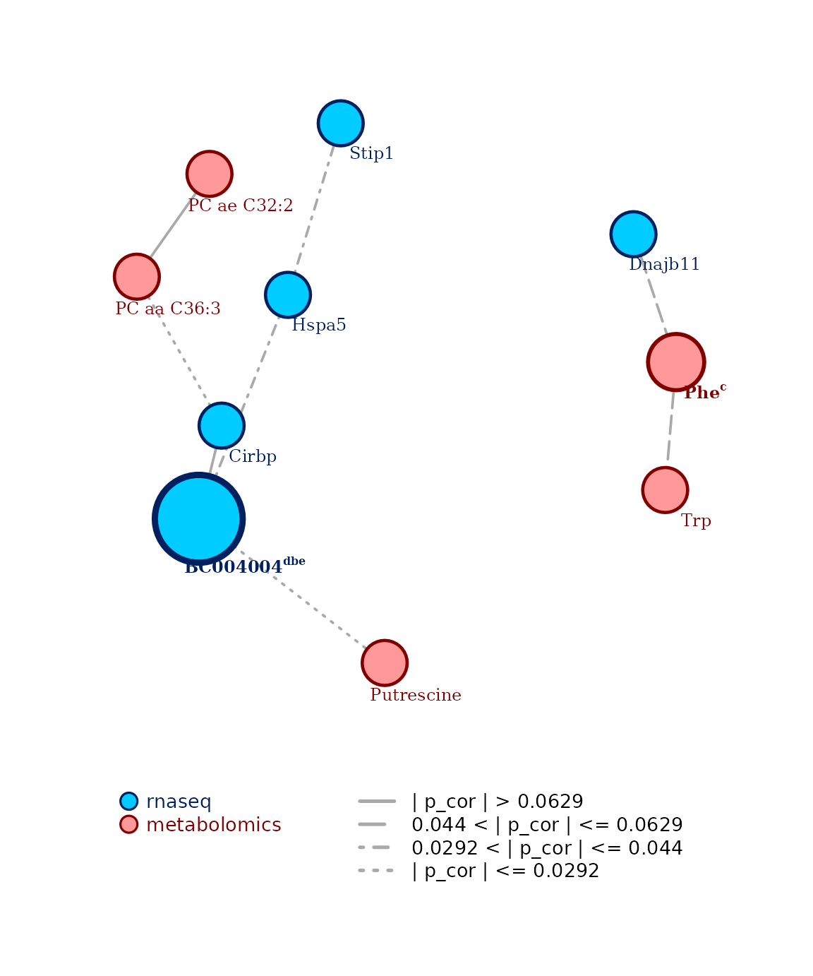
The second plot generated is the selected multi-omics network, enriched by the results of the centrality analysis when this one is performed. When an omics feature is found to be central according to a measure, the first letter of the measure is added at the end of the displayed node label, and the node itself is plotted larger. This also means that the larger the consensus, the larger the node will be. At the bottom of the plot, a legend shows the color coding for the different omics types of the network and the different edge types for the different edge strengths, depicting how strong the connection is. The multi-omics network plot can be personalized with three different arguments to carmon():

plot_hot_nodes can be set to FALSE to turn off the enrichment of the network based on the centrality analysis, and it is turned on by default.
plot_node_labels can be set to FALSE to hide the node labels from the plot, which is particularly useful for larger networks. When plot_hot_nodes is TRUE (default behavior) and plot_node_labels is FALSE, only the central nodes’ labels are displayed in the plot.
hide_isolated hides the unconnected nodes from the plot of the multi-omics network, TRUE by default.

Please note that also the plotting module can be turned off by setting the argument to carmon() plot = FALSE.

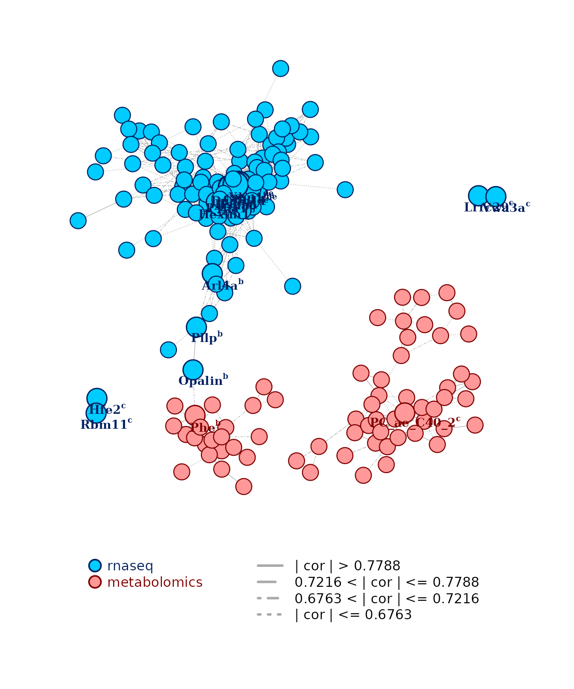
Custom run of `carmon()`

In this run, we customize the default behavior of carmon() with the information provided above, this time reconstructing the network from the largest data set provided by the package, multi_omics. We will will use alternative marginals for the RNA-seq layer, keeping the default for the metabolomic layer. We will use the omics features in the normal-realm to build a network with Pearson’s correlation, selecting only the top 5% connections. We will perform the consensus centrality analysis with all four measures, but we will select the top 2% for each measure to select the candidates for consensus. Moreover, we will hide the name of those nodes that are not found to be central. Finally, we will inspect the result of the consensus centrality analysis.

data(multi_omics)
str(multi_omics) # 162 genes, 76 metabolites, for 30 observations
#> List of 2
#>  $ rnaseq      : num [1:30, 1:162] 407 54 148 269 76 91 500 482 65 201 ...
#>   ..- attr(*, "dimnames")=List of 2
#>   .. ..$ : chr [1:30] "BXD100" "BXD101" "BXD73b" "BXD44" ...
#>   .. ..$ : chr [1:162] "Plin4" "Arc" "Egr2" "Tekt4" ...
#>  $ metabolomics: num [1:30, 1:76] 317 208 255 282 362 ...
#>   ..- attr(*, "dimnames")=List of 2
#>   .. ..$ : chr [1:30] "BXD100" "BXD101" "BXD73b" "BXD44" ...
#>   .. ..$ : chr [1:76] "Ala" "Arg" "Asn" "Cit" ...

c_obj <- carmon(multi_omics,
    marginals = c("e", 0), # Sets the empirical marginal distribution
    # for the first layer, and the default
    # distribution for the second
    net_method = "correlation", # Selecting Pearson's correlation
    cor_quant = 0.05, # Selecting the top 5% of connections
    quantile_c_measures = 0.02, # Top 2% of the candidates
    # to determine consensus of centrality
    plot_node_labels = FALSE
)
#> Checking sample-matching, formatting the data,
#>     and other formalities....
#> Done!
#> ****************Beginning copulization****************
#> Copulizing layer 1 of 2 (rnaseq)
#> Copulizing layer 2 of 2 (metabolomics)
#> ****************Copulization complete*****************
#> ***********Beginning network reconstruction***********
#> Reconstructing network with Pearson's correlation....
#> Correlation cutoff is 0.64002200550331
#> Network reconstructed!
#> ***********Network reconstruction complete************
#> **************Beginning network analysis**************
#> Computing centrality measures....
#> Centrality measures computed!
#> Compiling the report....
#> Report compiled!
#> **************Network analysis complete***************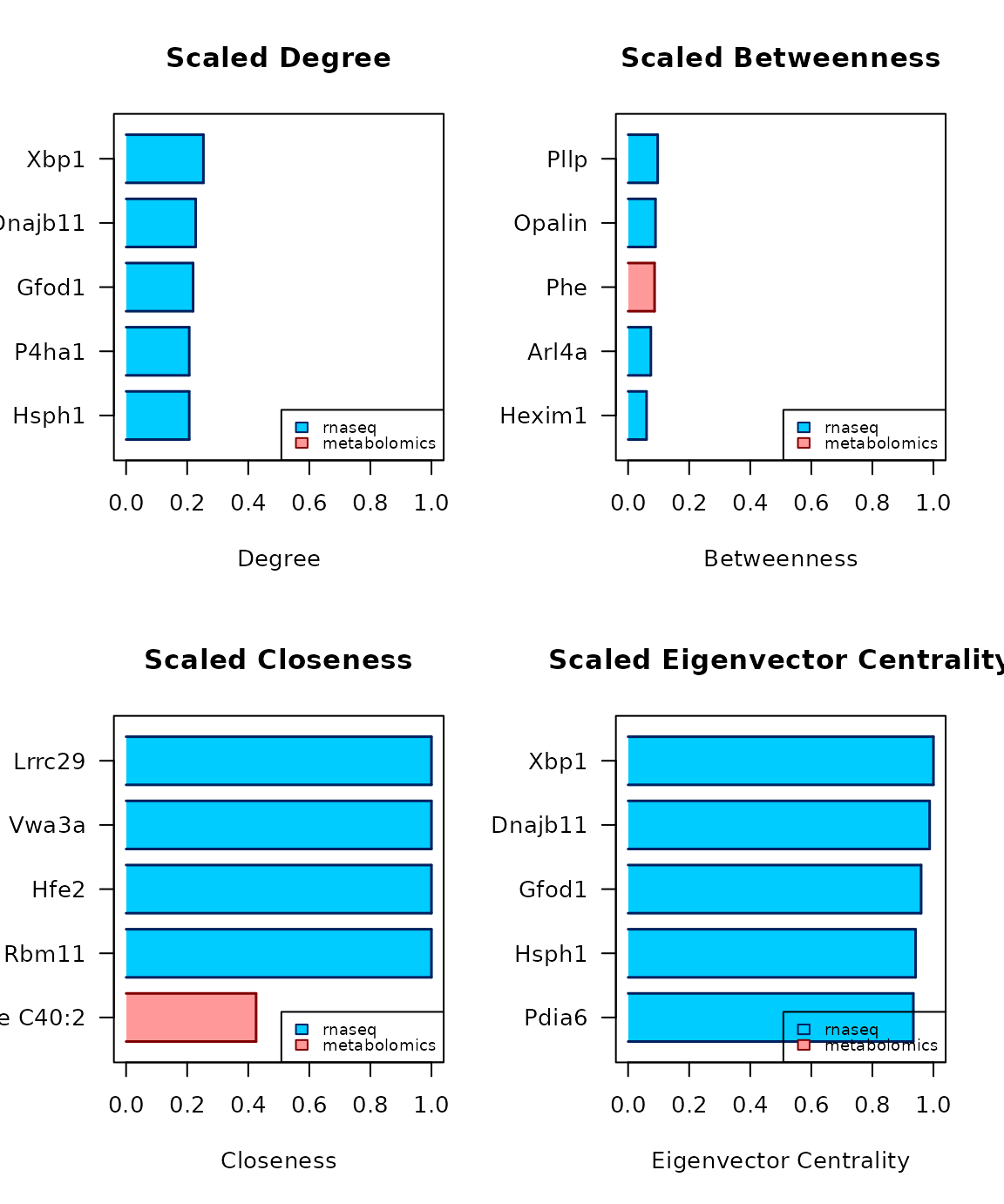


centrality_report(c_obj)
#>               candidate  degree betweenness closeness eigenvector central for
#> Xbp1               Xbp1 0.2532*      0.0226    0.4072          1*          de
#> Dnajb11         Dnajb11 0.2278*      0.0076    0.3965     0.9875*          de
#> Gfod1             Gfod1 0.2194*      0.0062    0.3908     0.9597*          de
#> Hsph1             Hsph1 0.2068*      0.0045    0.3886     0.9415*          de
#> Pdia6             Pdia6  0.1983      0.0032    0.3853     0.9342*           e
#> P4ha1             P4ha1 0.2068*      0.0054    0.3853      0.9007           d
#> Hexim1           Hexim1  0.1899     0.0604*    0.4159      0.8308           b
#> Lrrc29           Lrrc29  0.0042           0        1*           0           c
#> Vwa3a             Vwa3a  0.0042           0        1*           0           c
#> Hfe2               Hfe2  0.0042           0        1*           0           c
#> Rbm11             Rbm11  0.0042           0        1*           0           c
#> PC ae C40:2 PC ae C40:2  0.0717      0.0107   0.4257*           0           c
#> Arl4a             Arl4a   0.038     0.0745*      0.34      0.0542           b
#> Pllp               Pllp  0.0211     0.0969*    0.2804      0.0025           b
#> Opalin           Opalin  0.0084     0.0897*    0.2361       1e-04           b
#> Phe                 Phe  0.0422     0.0867*    0.2033           0           b

A note on input data formatting

It is also possible to provide carmon() with a single unified multi-omics data set, but then it is necessary to specify the argument p, a vector with the number of features of each layer, in the same order as the layers are assembled in the data set. Moreover, with this use case we strongly recommend using the omics argument to specify which omics type is measured by each layer. To see which omics types carmon() is tailored for, together with their accepted synonyms and assumed statistical behavior, see which_omics().

References

Albanese, A., Kohlen, W., & Behrouzi, P. (2024). Collaborative graphical lasso (arXiv:2403.18602). arXiv https://doi.org/10.48550/arXiv.2403.18602

Friedman, J., Hastie, T., & Tibshirani, R. (2008). Sparse inverse covariance estimation with the graphical lasso. Biostatistics, 9(3), 432–441. https://doi.org/10.1093/biostatistics/kxm045

Meinshausen, N., & Buhlmann, P. (2006). High-dimensional graphs and variable selection with the Lasso. Ann. Statist., 34(3), 1436-1462. https://doi.org/10.1214/009053606000000281

Liu, H., Roeder, K., & Wasserman, L. (2010). Stability Approach to Regularization Selection (StARS) for High Dimensional Graphical Models (arXiv:1006.3316). arXiv https://doi.org/10.48550/arXiv.1006.3316

Session Info

sessionInfo()
#> R version 4.5.1 (2025-06-13)
#> Platform: x86_64-pc-linux-gnu
#> Running under: Ubuntu 24.04.3 LTS
#> 
#> Matrix products: default
#> BLAS:   /usr/lib/x86_64-linux-gnu/openblas-pthread/libblas.so.3 
#> LAPACK: /usr/lib/x86_64-linux-gnu/openblas-pthread/libopenblasp-r0.3.26.so;  LAPACK version 3.12.0
#> 
#> locale:
#>  [1] LC_CTYPE=C.UTF-8       LC_NUMERIC=C           LC_TIME=C.UTF-8       
#>  [4] LC_COLLATE=C.UTF-8     LC_MONETARY=C.UTF-8    LC_MESSAGES=C.UTF-8   
#>  [7] LC_PAPER=C.UTF-8       LC_NAME=C              LC_ADDRESS=C          
#> [10] LC_TELEPHONE=C         LC_MEASUREMENT=C.UTF-8 LC_IDENTIFICATION=C   
#> 
#> time zone: UTC
#> tzcode source: system (glibc)
#> 
#> attached base packages:
#> [1] stats     graphics  grDevices utils     datasets  methods   base     
#> 
#> other attached packages:
#> [1] carmon_0.99.0    BiocStyle_2.36.0
#> 
#> loaded via a namespace (and not attached):
#>  [1] SummarizedExperiment_1.38.1 gtable_0.3.6               
#>  [3] xfun_0.53                   bslib_0.9.0                
#>  [5] ggplot2_4.0.0               Biobase_2.68.0             
#>  [7] lattice_0.22-7              vctrs_0.6.5                
#>  [9] tools_4.5.1                 generics_0.1.4             
#> [11] stats4_4.5.1                parallel_4.5.1             
#> [13] pkgconfig_2.0.3             Matrix_1.7-3               
#> [15] RColorBrewer_1.1-3          S7_0.2.0                   
#> [17] desc_1.4.3                  S4Vectors_0.46.0           
#> [19] lifecycle_1.0.4             GenomeInfoDbData_1.2.14    
#> [21] compiler_4.5.1              farver_2.1.2               
#> [23] textshaping_1.0.4           DESeq2_1.48.2              
#> [25] codetools_0.2-20            GenomeInfoDb_1.44.3        
#> [27] htmltools_0.5.8.1           sass_0.4.10                
#> [29] yaml_2.3.10                 pkgdown_2.1.3              
#> [31] crayon_1.5.3                jquerylib_0.1.4            
#> [33] BiocParallel_1.42.2         cachem_1.1.0               
#> [35] DelayedArray_0.34.1         abind_1.4-8                
#> [37] locfit_1.5-9.12             digest_0.6.37              
#> [39] bookdown_0.45               fastmap_1.2.0              
#> [41] grid_4.5.1                  cli_3.6.5                  
#> [43] SparseArray_1.8.1           magrittr_2.0.4             
#> [45] S4Arrays_1.8.1              withr_3.0.2                
#> [47] UCSC.utils_1.4.0            scales_1.4.0               
#> [49] rmarkdown_2.30              XVector_0.48.0             
#> [51] httr_1.4.7                  matrixStats_1.5.0          
#> [53] igraph_2.2.1                ragg_1.5.0                 
#> [55] evaluate_1.0.5              knitr_1.50                 
#> [57] GenomicRanges_1.60.0        IRanges_2.42.0             
#> [59] rlang_1.1.6                 Rcpp_1.1.0                 
#> [61] glue_1.8.0                  BiocManager_1.30.26        
#> [63] BiocGenerics_0.54.1         jsonlite_2.0.0             
#> [65] R6_2.6.1                    MatrixGenerics_1.20.0      
#> [67] systemfonts_1.3.1           fs_1.6.6                   
#> [69] coglasso_1.1.0

Alessio Albanese